From this chapter, you start to learn how to use MBDyn by actually writing input files and running MBDyn through example problems. Since this tutorial is not meant to cover all aspects of MBDyn's input format and syntax, please refer to the official "Input manual," which can be obtained at the MBDyn site, for details about the input format and syntax. There is also the official "Tutorials" at the site, which is worth looking at as well. Our first example is similar to an example treated in the official Tutorials.

Problem 1 (Free-falling body)

Simulate the motion of a body with mass of 1.0kg that is thrown horizontally with an initial speed of 3.0m/s and is under the influence of gravity alone. Suppose the gravity acceleration is 9.81m/s².

Global reference frame

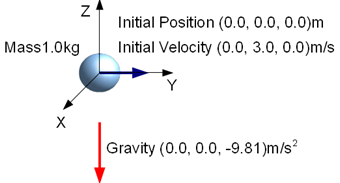
When we conduct an analysis with MBDyn, we first have to define the global (or absolute) reference frame in which a simulation model is constructed and its motion is described. Since the global reference frame can be defined arbitrarily as long as it is at rest, we should define it in a way it is convenient for us. For Problem 1, let us define the global reference frame with its origin at the initial position of the center of mass of the body, its Z-axis pointing upward, and its Y-axis in the direction of the initial velocity of the body. (See Figure 1.)

Flow of MBDyn analysis

In this tutorial we shall call the series of processes for simulating the motion of a multibody system with MBDyn "MBDyn analysis" or simply "analysis." The general flow of an MBDyn analysis is shown in Figure 2.

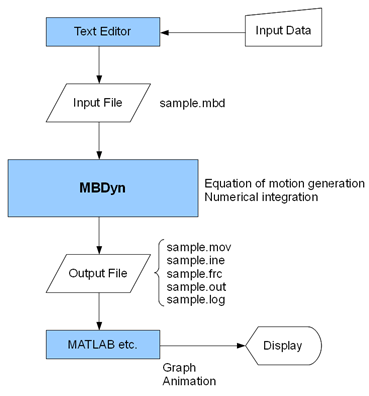
First, the user creates an input file with a text editor. The user writes input data into the input file in a specific format. The extension of the input file is arbitrary, but we shall use ".mbd" in this tutorial. Next, the user runs MBDyn with the input file specified. Then, MBDyn reads the input file, generates the equations of motion, and computes the motion of the subject system. If everything goes fine, MBDyn writes the result into some output files. If a problem occurs in midstream, MBDyn stops its process and issues an error message, in which case the input file needs to be amended so that the cause of the error is eliminated.

The output files contain the data of the simulated motion of the subject system such as position, velocity, orientation, and angular velocity of each rigid body and joint reaction forces. The user may import this data in numerical analysis software such as MATLAB and make graphs and animations to visualize the simulated motion. This is called post-processing.

Now, let's follow the flow of the MBDyn analysis for Problem 1.

Input file

An example input file for the analysis of Problem 1 is shown in Code 1. The code is analyzed in detail in the next two chapters. But for now, without any explanation, let's look through it and guess what is written.

# free_falling_body.mbd

begin: data;
   problem: initial value;
end: data;
 
begin: initial value;
   initial time: 0.;
   final time: 1.;
   time step: 1.e-3;
   max iterations: 10;
   tolerance: 1.e-6;
end: initial value;
 
begin: control data;
   structural nodes: 1;
   rigid bodies: 1;
   gravity;
end: control data;
 
begin: nodes;
   structural: 1, dynamic, null, eye, 0., 3., 0., null;
end: nodes;
 
begin: elements;
   body: 1, 1, 1., null, eye;
   gravity: 0., 0., -1., const, 9.81;
end: elements;

Running MBDyn

Let's run MBDyn with the above input file. First, save the input file of Code 1 in the current directory with the name "free_falling_body.mbd." Then, in a shell, invoke

   mbdyn -f free_falling_body.mbd

MBDyn will be executed and a message like the following will appear.

MBDyn - MultiBody Dynamics 1.X-Devel
compiled on Nov  1 2009 at 16:57:21

Copyright 1996-2009 (C) Paolo Mantegazza and Pierangelo Masarati,
Dipartimento di Ingegneria Aerospaziale <http://www.aero.polimi.it/>
Politecnico di Milano                   <http://www.polimi.it/>

MBDyn is free software, covered by the GNU General Public License,
and you are welcome to change it and/or distribute copies of it
under certain conditions.  Use 'mbdyn --license' to see the conditions.
There is absolutely no warranty for MBDyn.  Use "mbdyn --warranty"
for details.

reading from file "free_falling_body.mbd"
Creating scalar solver with Naive linear solver
Reading Structural(1)
Reading Body(1)
Reading Gravity
No initial assembly is required since no joints are defined
End of simulation at time 1 after 1000 steps;
output in file "free_falling_body.mbd"
total iterations: 298
total Jacobian matrices: 298
total error: 0.000328629
MBDyn terminated normally

The above message implies that MBDyn completed its process without any problem. Several output files with the name "free_falling_body.<extension>" will be created in the current directory. In our present case, output files with the extensions "out", "log", "mov", "ine" will be generated. The files with the extensions "out" and "log" will contain general information about the simulation. The files with the extensions "mov" and "ine" will contain the time-series data of the motion of each rigid body such as position and velocity. You may want to check the output data by actually opening those files.

Visualization of simulation result

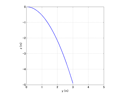
The data written into the output files are of course mere arrays of numbers. In order to see the result of a simulation it is often necessary to visualize the numerical data. Two examples of visualization of the simulation result for Problem 1 are shown in Figure 3 and Movie 1.

Figure 1 shows a graph of the trajectory of the body and Movie 1 shows an animation of the motion of the body. Both are made from the data written in the mov file. From these graph and animation we can visually see that the body falls along a parabolic curve. Some techniques to make graphs and animations by processing the output data are discussed in the later chapters.