This chapter explains the basics of how to handle MBDyn output data.
A result of an MBDyn analysis is usually written into some output files. If we run MBDyn with the input file "free_falling_body.mbd," the following four output files are generated.
Among them, the files with the extensions "out" and "log" contain general information about the simulation and the files with the extensions "mov" and "ine" contain the time-series data of the motions of rigid bodies. The mov file contains data of position, orientation, velocity, and angular velocity of each structural node. The ine file contains data of momentum, angular momentum, and their derivatives of each rigid body.
Figure 1 shows the data of the mov file "free_falling_body.mov" displayed with spreadsheet software. It is actually simple space-separated numerical data in ASCII format.
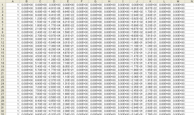
Data in a mov file is generally formatted as follows.
These quantities are basically with respect to the global reference frame. The number of rows is equal to the product of the number of nodes and the number of time steps. In our current example, since there is only one node, there is an output of only one row at each time step. In a general case, if there are N nodes, there is an output of N rows corresponding to the N nodes at each time step.
Orientations are expressed in terms of xyz Euler angles. An orientation with the xyz Euler angles (α,β,γ) is the orientation obtained by consecutive rotations about x, y, and z axies of the body-fixed frame by angles α, β, and γ, in this order. The relationship between the xyz Euler angles (α,β,γ) and the orientation matrix R is given by
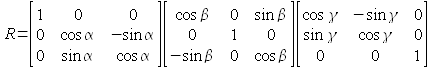
The expression of orientation in the mov file can be changed by using the "default orientation" card in the control data block as
default orientation: { euler123 | orientation vector | orientation matrix } ;
where euler123 is the default xyz Euler angles. We have to keep in mind that if the default orientation is changed, then the number of columns the orientation data occupy in the mov file changes and the column indices for the velocity and angular velocity data also change.
Lastly, we note that the mov files does not include time data. If we need time data, we have to either create it according to the time step setting in the input file or refer to the out file.
In this tutorial, we proceed with the assumption that we use MATLAB for processing output data for the convenience of discussion. But similar processing can be carried out using other numerical analysis software such as Scilab and Octave. If you use other software, please interpret the MATLAB language in the following text into the language of the software you use.
Data in a mov file are space-separated numerical data in ASCII format. It can be imported to MATLAB using, for example, the dlmread command.
M = dlmread('free_falling_body.mov');
The matrix M will then contain the whole data in the mov file "free_falling_body.mov." By entering
x = M(:,2); y = M(:,3); z = M(:,4);
we get each component of the position. Similarly, by entering
vx = M(:,8); vy = M(:,9); vz = M(:,10);
we get each component of the velocity. (If there are multiple nodes, because each column contains data of more than one node, an additional process to separate data for each node is necessary. Processing of multiple-nodes data is treated in Chapter 11.)
Using these data vectors we can plot a variety of graphs. For example,
plot(y,z)
plots the trajectory of the body in the YZ plane. And
plot3(x,y,z)
lets us view the trajectory in a 3D frame.
To plot a graph with respect to time, we need a time vector. If we refer to the input file, we see the setting that the output is from time 0(s) to 1(s) with the step size 1e-3(s). So we can create a time vector as follows.
t = 0:1.e-3:1;
After creating the time vector, if we enter
plot(t,y)
we can plot the y-position of the body with respect to time.
Post-processing is not just about plotting graphs. We may want to extract some information from output data. For example, the z-position of the body at time 0.1(s) can be obtained as follows.
z_01 = z(min(find(t>=0.1)));
As another example, the time at which the z-position of the body reaches -1(m) can be obtained by
t1 = t(min(find(z<-1)));
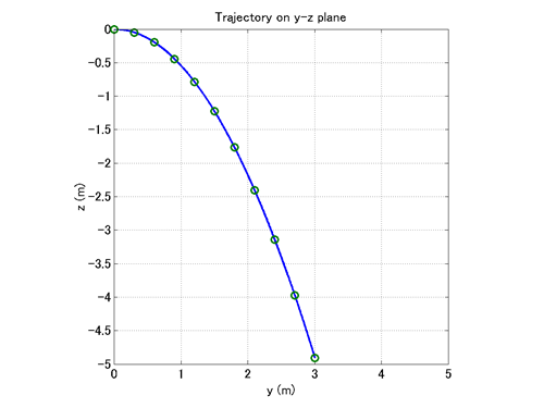
Finally, we present a MATLAB script in Code 1 that draws the trajectory of the body as well as markers that indicate the position of the body at every 0.1(s). Figure 2 shows the graph drawn by this script.
% plot_trajectory.m

clear; close all;

M = dlmread('free_falling_body.mov');

x = M(:,2); y = M(:,3); z = M(:,4);

t = 0:1.e-3:1;

td = 0:0.1:1;

for k=1:length(td)
    yd(k) = y(min(find(t>=td(k))));
    zd(k) = z(min(find(t>=td(k))));
end

plot(y,z,'-',yd,zd,'o','LineWidth',2,'MarkerSize',8);
grid on;
axis([0,5,-5,0]);
axis square;
xlabel('y (m)','FontSize',14);
ylabel('z (m)','FontSize',14);
title('Trajectory on y-z plane','FontSize',14);
set(gca,'FontSize',14);