When an MBDyn analysis is carried out on a model that includes joints, an additional output file with the extension "jnt" (jnt file) is generated. A jnt file contains data of joint reaction forces and some extra data depending on the type of joint. In this chapter we discuss how to handle joint output data using the jnt file obtained by the MBDyn analysis of Problem 4 in the previous chapter.

Format of jnt file

Figure 1 shows the data in the jnt file "double_rigid_pendulum_2.jnt" obtained by the MBDyn analysis of Problem 4.

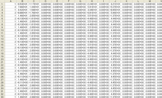
In general, data in a jnt file consist of two parts: the standard part that is common to all joints and the extra part that depends on the type of joint. The standard part is the first 13 columns and is formatted as follows.

• Column 1: Joint label
• Column 2-4: Components of the reaction force in a local frame
• Column 5-7: Components of the reaction couple (torque) in a local frame
• Column 8-10: Components of the reaction force in the global frame
• Column 11-13: Components of the reaction couple (torque) in the global frame

In Figure 1, we can see that the data of joint "1" and joint "2" are written alternately row by row. In fact, when there are two joints, at each time step there is an output of two rows corresponding to the two joints. Generally, when there are N joints, at each time step there is an output of N rows corresponding to the N joints.

Since the format of a jnt file is similar to the format of a mov file we saw in Chapter 11, we can use the MATLAB function "MBDynLoad" introduced in Chapter 11 to process jnt files as well.

Reaction force of revolute pin

Let's import the jnt file "double_rigid_pendulum_2.jnt" in MATLAB and plot the reaction force of the revolute pin.

First, we import the data of "double_rigid_pendulum_2.jnt" using the function "MBDynLoad."

[LABEL,DATA] = MBDynLoad('double_rigid_pendulum_2.jnt');

Next, noting that the label of the revolute pin is "1," we make data vectors of the components of the reaction force of the revolute pin as follows.

f1x = DATA(:,2,LABEL==1);
f1y = DATA(:,3,LABEL==1);
f1z = DATA(:,4,LABEL==1);

F1x = DATA(:,8,LABEL==1);
F1y = DATA(:,9,LABEL==1);
F1z = DATA(:,10,LABEL==1);

Here, (f1x, f1y, f1z) is the representation of the reaction force in the local reference frame and (F1x, F1y, F1z) is the representation of the reaction force in the global reference frame. The local reference frame of the revolute pin is the reference frame defined by the hinge in the statement that defines the revolute pin and fixed to the Link1.

Meanwhile, the time data vector can be created as follows.

t = 1.e-3*[0:length(f1x)-1]';

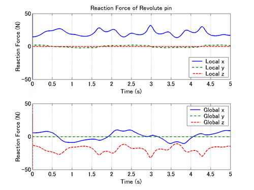
Using these data vectors, we can plot the components of the reaction force of the revolute pin with respect to time as follows, for example. The resulting graph is shown in Figure 2.

figure(1)

subplot(2,1,1)
plot(t,f1x,t,f1y,'-.',t,f1z,'--')

subplot(2,1,2)
plot(t,F1x,t,F1y,'-.',t,F1z,'--')

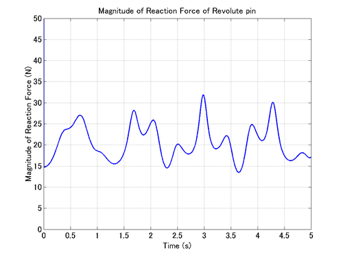
Next, let's examine the magnitude of the reaction force of the revolute pin. The magnitude of the reaction force is obtained by the square root of the sum of the squares of the components of the reaction force, and therefore we can create the data vector of the magnitude of the reaction force as follows.

f1 = sqrt(f1x.^2+f1y.^2+f1z.^2);

Then, we can plot the magnitude of the reaction force of the revolute pin as follows. The resulting graph is shown in Figure 3.

figure(2)
plot(t,f1)

In the above, the magnitude of the reaction force is obtained from the three components in the local reference frame, but since the magnitude of the reaction force does not depend on a reference frame, we can obtain the same result with the three components in the global reference frame.

Revolute pin/hinge extra data

A jnt file may include extra data depending on the type of joint in addition to the standard data in the first 13 columns. In the case of revolute pin/hinge, the following extra data is available.

• Column 14-16: Euler angles (in degrees) that describe the relative rotation; only the third component is relevant, the first two essentially indicate the accuracy of the rotation constraint
• Column 17-19: the relative angular velocity

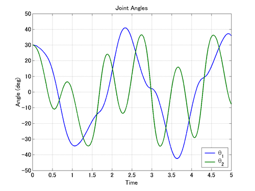
Now, let's plot θ₁ and θ₂ using this extra data. This can be done with the script shown in Code 1 (in the case when initial angles θ₁ and θ₂ are both π/6(=30deg)). The graph drawn by this script is shown in Figure 4.

% plot_theta.m

clear; close all;

[LABEL,DATA] = MBDynLoad('double_rigid_pendulum_2.jnt');

a1z = DATA(:,16,LABEL==1);
a2z = DATA(:,16,LABEL==2);

t = 1.e-3*[0:length(a1z)-1]';

theta1 = 30-a1z;
theta2 = 30-a2z;

plot(t,theta1,t,theta2,'LineWidth',1.5)
grid on;
set(gca,'FontSize',14);
xlabel('Time','FontSize',14);
ylabel('Angle (deg)','FontSize',14);
title('Joint Angles');
legend('\theta_1','\theta_2',0);