In this chapter we consider a new example problem. Like the last problem, we consider an extremely simple model. While in the last problem we dealt with a translational motion, in the new problem here we deal with rotational motions.
In a space without gravity, we consider a rectangular block as shown in Figure 1. The mass of the block is M=1.0kg and the length, width, and height of the block are Lx=15cm, Ly=5cm, and Lz=30cm, respectively. Create an input file to simulate the motion of the block when arbitrary initial angular velocity is given.
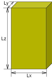
We define the global reference frame such that its origin is at the center of mass of the block and its X, Y, and Z axes are parallel to Lx, Ly, and Lz, respectively, at initial time. The principal axes of inertia coincide with the global frame axes at the initial time and the principal moments of inertia are given by the following equations.

If we substitute the mass M and the lengths Lx, Ly, and Lz in these equations, we obtain Ixx=7.7e-3(kg m2), Iyy=9.4e-3(kg m2), and Izz=2.1e-3(kg m2) and we observe that Iyy > Ixx > Izz.
An example input file for Problem 2 is shown in Code 1 below.
# free_rotating_block.mbd

begin: data;
   problem: initial value;
end: data;

begin: initial value;
   initial time:   0.;
   final time:     5.;
   time step:      1.e-2;
   max iterations: 10;
   tolerance:      1.e-6;
end: initial value;

begin: control data;
   structural nodes: 1;
   rigid bodies:     1;
end: control data;

# Design Variables
set: real M   = 1.;   # [kg] Mass
set: real Lx  = 0.15; # [m] Width
set: real Ly  = 0.05; # [m] Thickness
set: real Lz  = 0.3;  # [m] Height
set: real Wx0 = 0.;   # [rad/s] Initial angular velocity along x axis
set: real Wy0 = 0.;   # [rad/s] Initial angular velocity along y axis
set: real Wz0 = 5.;   # [rad/s] Initial angular velocity along z axis

set: real Ixx = 1./12.*M*(Ly^2+Lz^2); # [kgm^2] Moment of inertia about x axis
set: real Iyy = 1./12.*M*(Lz^2+Lx^2); # [kgm^2] Moment of inertia about y axis
set: real Izz = 1./12.*M*(Lx^2+Ly^2); # [kgm^2] Moment of inertia about z axis

# Node Labels
set: integer Node_Block = 1;

# Body Labels
set: integer Body_Block = 1;

begin: nodes;
   structural: Node_Block, dynamic,
      0., 0., 0.,    # absolute position
      eye,           # absolute orientation
      null,          # absolute velocity
      Wx0, Wy0, Wz0; # absolute angular velocity

end: nodes;

begin: elements;
   body: Body_Block, Node_Block,
      M,                   # mass
      null,                # relative center of mass
      diag, Ixx, Iyy, Izz; # inertia matrix

end: elements;
First, note how the inertia matrix of the block is defined. This is done in three steps. The first step is to define M, Lx, Ly, and Lz as design variables using the set card. The second step is to calculate Ixx, Iyy, and Izz from the design variables by the equations given above (the set card is used here, too). The final step is to define the inertia matrix of the body "Body_Block" in terms of Ixx, Iyy, and Izz. The inertia matrix for "Body_Block" is defined as follows.
diag, Ixx, Iyy, Izz
where "diag" is the keyword to define a diagonal matrix with three values that follow as diagonal elements. By the way, a general inertia matrix is a symmetric matrix and can be defined using the keyword "sym." (See Chapter 12.)
Next, note that the initial angular velocity of the node "Node_Block" is defined with the design variables Wx0, Wy0, and Wz0. Because we want to simulate the motion of the block with arbitrary initial angular velocity, it is convenient to define the initial angular velocity as a variable.
Let us simulate the motion of the block for the three cases below.
Movies 1-3 show animations of the simulation results. In Case 1 the block rotates around the principal axis corresponding to the Z-axis, while in Case 2 it rotates around the principal axis corresponding to the X-axis. In Case 3 the block exhibits a more general rotational motion.