Chapter 7 explained the basics of how to handle output data in a mov file. But the example treated in Chapter 7 was rather a special case where there was only one node. In this chapter, we discuss how to handle output data in a mov file in a general case where there are multiple nodes

Format of mov file with multiple nodes

In the input file "free_rotating_block_dummynode.mbd" given in the last chapter, there are two nodes including a dummy node. Figure 1 shows the data in the mov file obtained by an MBDyn analysis with this input file.

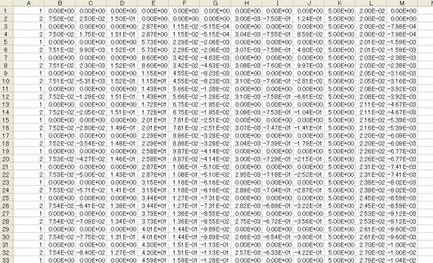
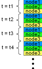
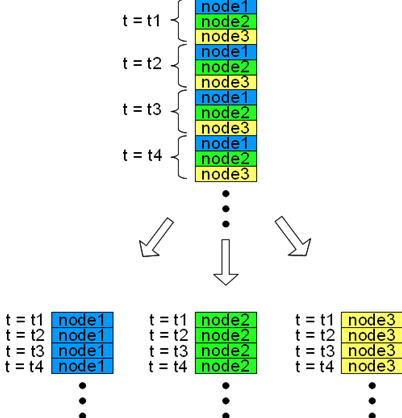
The first column of a mov file contains node labels (see Chapter 7). In Figure 1 we can see that the data of node "1" and node "2" are written alternately row by row. In fact, when there are two nodes, at each time step there is an output of two rows corresponding to the two nodes. Generally, when there are N nodes, at each time step there is an output of N rows corresponding to the N nodes. (See Figure 2.)

Separation of data for each node

When there are multiple nodes, since each column of the mov file contains data of multiple nodes, we cannot make graphs and so on using the raw column data as is as in Chapter 7. In this case, we need an additional process to separate the data for each node as shown schematically in Figure 3.

Post-processing with MATLAB

A simple program can carry out the process illustrated in Figure 3. The link below is an M-file for a convenient MATLAB function (and similar programs for other software) that reads a mov file and carry out the process illustrated in Figure 3.

MBDynLoad.m (for MATLAB)

MBDynLoad.sci (for Scilab)

MBDynLoad2.m (for Octave)

This MATLAB function "MBDynLoad" is used as follows.

   [LABEL,DATA] = MBDynLoad(FILENAME);

If we enter the above line of commands with an existing mov file in place of FILENAME, node labels are stored in LABEL and the reorganized data are stored in DATA as a three dimensional array. The value of DATA(i,j,k), with i, j, and k being natural numbers, is the value of the jth column at the ith time step of the kth node (not the node with label "k", though).

For example, if "sample.mov" is a mov file and we enter

   [LABEL,DATA] = MBDynLoad('sample.mov');

and

   x = DATA(:,2,LABEL==5);

then we obtain a time-series data vector for the x component of the position of the node "5".

By the way, the function "MBDynLoad" is applicable to other output data files than mov files such as ine, frc, and jnt files.

Trajectory of the block corner

Now, let's plot the trajectory of the corner of the block for our current example problem. Code 1 shows a MATLAB script that reads "free_rotating_block_dummynode.mov" and plots the position of the node "2" (the dummy node attached to the corner of the block) in a 3D frame. ("MBDynLoad" is used in the script)

% plot_dummynode_trajectory.m

clear; close all;

[LABEL,DATA]=MBDynLoad('free_rotating_block_dummynode.mov');

x=DATA(:,2,LABEL==2);
y=DATA(:,3,LABEL==2);
z=DATA(:,4,LABEL==2);

plot3(x,y,z,'LineWidth',1)
grid on;
axis([-0.2,0.2,-0.2,0.2,-0.2,0.2]);
axis vis3d;
set(gca,'FontSize',12);
xlabel('x (m)','FontSize',12);
ylabel('y (m)','FontSize',12);
zlabel('z (m)','FontSize',12);
title('Trajectory of the block corner','FontSize',12);

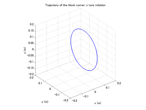
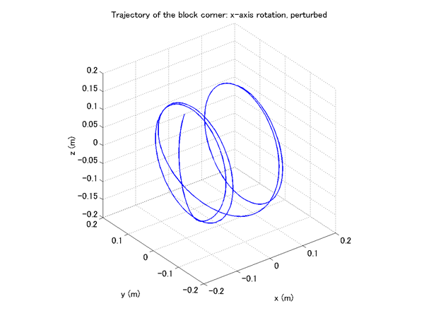
Figure 4 and 5 show the trajectories of the corner of the block for the following two cases.

• Case 1: Wx0=5., Wy0=0., Wz0=0. (rad/s)
• Case 2: Wx0=5., Wy0=0.02, Wz0=0. (rad/s)

In Case 1, the block rotates about the X-axis and the trajectory of the corner is a circle. In Case 2, because of the instability of rotation about the X-axis, the axis of rotation deviates largely from the X-axis and the corner of the block traces a complex path.