This chapter introduces the fundamental idea of animation and explains how to make an animation of a rigid body motion from MBDyn output data.
First, we consider a simple one-dimensional case to illustrate the fundamental idea of animation.
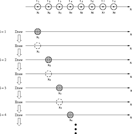
Suppose a point moves on the x-axis with time. If the positions of the point are given for a fixed time interval as x = x1, x2, x3, ... then an animation of the moving point can be made by looping the following 1-3. Assume the point is represented by a small circle. (See Figure 1.)
Code 1 below is an example MATLAB script that makes such an animation of a moving point. The animation made by this script is shown in Movie 1.
% animation_point.m

clear; close all;

% Create data
t = 0:0.001:1;   % Time data
x = sin(2*pi*t); % Position data

% Draw initial figure
figure(1);
set(gcf,'Renderer','OpenGL');
h = plot(x(1),0,'o','MarkerSize',20,'MarkerFaceColor','b');
set(h,'EraseMode','normal');
xlim([-1.5,1.5]);
ylim([-1.5,1.5]);

% Animation Loop
i = 1;
while i<=length(x)
    set(h,'XData',x(i));
    drawnow;
    i = i+1;
end
The fundamental idea is the same for an animation of a rigid body motion. The only difference is that in the case of a rigid body motion the object to draw and erase is a three-dimensional shape. Since MBDyn describes a motion of a rigid body in terms of a motion of a node, a process to convert motion data of a node to motion data of a shape is required.
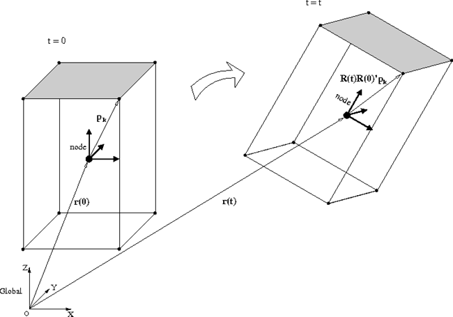
For example, let's consider a case where the shape is a block as in Figure 2. First, we define the vertices of the block at the initial time (see the left hand side of Figure 2). Since the shape of the block moves with the node and the relative positions of the vertices with respect to the node are invariant, the positions of the vertices at an arbitrary time can be calculated from the position and the orientation of the node as illustrated in the right hand side of Figure 2. Once the positions of the vertices are obtained, the shape of the block can be drawn. In this way, if we calculate the positions of vertices at each time instance from the node data and go through the loop of drawing and erasing for the shape of the block, we can make an animation of the block.
To create a general three-dimensional shape in MATLAB, "patch" may be used. A patch is a polygonal surface defined by three or more vertex points. By putting together patches, we can create an arbitrary polyhedron. For example, a block shape can be made of six rectangular patches.
Code 2 below is a MATLAB script that reads the mov file obtained by the MBDyn analysis of the free-rotating block in Problem 2 and creates an animation of only the top patch of the block. The animation made by this script is shown in Movie 2. If we combine such animations for six patches, we can make an animation of the full block.
% animation_patch.m

clear; close all;

% Define Geometry Points (Vertices for the top surface of the block)
Lx = 0.15; %[m]
Ly = 0.05; %[m]
Lz = 0.30; %[m]

p1 = [  Lx/2,  Ly/2, Lz/2 ];
p2 = [  Lx/2, -Ly/2, Lz/2 ];
p3 = [ -Lx/2, -Ly/2, Lz/2 ];
p4 = [ -Lx/2,  Ly/2, Lz/2 ];

% Load Data
[LABEL,DATA] = MBDynLoad('free_rotating_block.mov');

r = DATA(:,[2:4],LABEL==1);        % Node Position [m]
A = DATA(:,[5:7],LABEL==1)*pi/180; % Node Orientation [rad] (x-y-z Euler angle)

n = size(r,1); % Data Length

% Euler Angle -> Orientation Matrix
for i=1:n
    a1 = A(i,1);
    a2 = A(i,2);
    a3 = A(i,3);

    R1 = [1, 0, 0;
        0, cos(a1), -sin(a1);
        0, sin(a1), cos(a1)];

    R2 = [cos(a2), 0, sin(a2);
        0, 1, 0;
        -sin(a2), 0, cos(a2)];

    R3 = [cos(a3), -sin(a3), 0;
        sin(a3), cos(a3), 0;
        0, 0, 1];

    R(:,:,i) = R1*R2*R3;
end

% Compute Propagation of Geometry Points
for i=1:n
    r1(i,:) = r(i,:) + p1*R(:,:,1)*R(:,:,i)';
    r2(i,:) = r(i,:) + p2*R(:,:,1)*R(:,:,i)';
    r3(i,:) = r(i,:) + p3*R(:,:,1)*R(:,:,i)';
    r4(i,:) = r(i,:) + p4*R(:,:,1)*R(:,:,i)';
end

% Compile Data for Drawing Patch
PatchData_X = [r1(:,1),r2(:,1),r3(:,1),r4(:,1)];
PatchData_Y = [r1(:,2),r2(:,2),r3(:,2),r4(:,2)];
PatchData_Z = [r1(:,3),r2(:,3),r3(:,3),r4(:,3)];

% Draw Initial Figure
figure(1);
set(gcf,'Renderer','OpenGL');
h = patch(PatchData_X(1,:),PatchData_Y(1,:),PatchData_Z(1,:),'y');
set(h,'EraseMode','normal');
axis vis3d equal;
view([-37.5,30]);
camlight;
grid on;
xlim([-0.2,0.2]);
ylim([-0.2,0.2]);
zlim([-0.2,0.2]);

% Animation Loop
for i=1:n
    set(h,'XData',PatchData_X(i,:)');
    set(h,'YData',PatchData_Y(i,:)');
    set(h,'ZData',PatchData_Z(i,:)');
    drawnow;
end