In the last chapter we saw how to define and use scalar functions. Now, when we define a scalar function, how can we verify the scalar function to be as we intended? This chapter introduces one way to do it. The technique introduced here that uses "abstract node" and "genel:clamp" can be applied not only to visualize scalar functions but also to visualize any variables in the model.
An "abstract node" is a general scalar (one degree of freedom) node. It is defined in the nodes block as follows.
abstract: <node label>, algebraic,
   value, <initial value>;
A "clamp" of the "genel" elements forces one arbitrary degree of freedom to assume a value specified by a drive. It is defined in the elements block as follows.
genel: <label>,
   clamp,
      <clamped node>,
      <imposed value>;
where <imposed value> is specified by a drive caller.
If we want to visualize a defined scalar function f(x) in the domain -5 ≤ x ≤ 5, we perform an MBDyn analysis (initial value problem) from time 0 to 10 that evaluates and outputs x = Time - 5 and y = f(x) at each time step. To output the values of the variables x and y, we define abstract nodes and link them to the variables by means of genel:clamp. Code 1 below is an example input file to visualize the scalar function "myfunc2" in the last chapter.
# scalarfunc.mbd

#-----------------------------------------------------------------------------
# Scalar Function
scalar function: "myfunc2",
   cubicspline, do not extrapolate,
      -2.0, 0.0,
      -1.0, 0.0,
       0.0, 0.0,
       1.0, 1.0,
       2.0, 1.0,
       3.0, 1.0;

# X Range
set: real XL = -5.;  # Lower Limit
set: real XU = 5.;   # Upper Limit
set: real dX = 0.01; # Step

#-----------------------------------------------------------------------------
# [Data Block]

begin: data;
   problem: initial value;
end: data;

#-----------------------------------------------------------------------------
# [<Problem> Block]

begin: initial value;
   initial time:   0.;
   final time:     XU-XL;
   time step:      dX;
   max iterations: 10;
   tolerance:      1.e-6;
end: initial value;

#-----------------------------------------------------------------------------
# [Control Data Block]

begin: control data;
   abstract nodes: 2;
   genels:         2;
end: control data;

#-----------------------------------------------------------------------------
# Abstract Node Labels
set: integer NoAbs_X = 1;
set: integer NoAbs_Y = 2;

# Genel Labels
set: integer GeClamp_NoAbs_X = 1;
set: integer GeClamp_NoAbs_Y = 2;

#-----------------------------------------------------------------------------
# [Nodes Block]

begin: nodes;

   abstract: NoAbs_X, algebraic,
      value, XL;

   abstract: NoAbs_Y, algebraic,
      value, model::sf::myfunc2(XL);

end: nodes;

#-----------------------------------------------------------------------------
# Plugin Variable
set: [dof, X, NoAbs_X, abstract, algebraic];

#-----------------------------------------------------------------------------
# [Elements Block]

begin: elements;

   genel: GeClamp_NoAbs_X,
      clamp,
         NoAbs_X, abstract,
         string, "Time+XL";

   genel: GeClamp_NoAbs_Y,
      clamp,
         NoAbs_Y, abstract,
         string, "model::sf::myfunc2(X)";

end: elements;
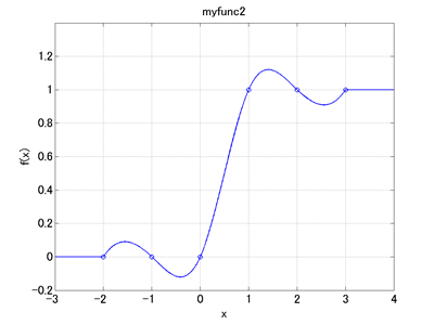
When we run MBDyn with Code 1 as the input file, a file named "scalarfunc.abs" is generated as output. This file stores the data for abstract nodes. The data in an abs file are composed of two columns where the first column contains the node labels and the second column contains the values of the abstract nodes. Code 2 below is a MATLAB script that reads the data of "scalarfunc.abs" and plots the scalar function "myfunc2" (See Chapter 11 for "MBDynLoad" function in the code). This script will give us a graph as shown in Figure 1.
% plot_scalarfunc.m

clear; close all;

[LABEL,DATA] = MBDynLoad('scalarfunc.abs');

X = DATA(:,2,LABEL==1);
Y = DATA(:,2,LABEL==2);

Xd = [-2, -1, 0, 1, 2, 3];
Yd = [0, 0, 0, 1, 1, 1];

figure(1)
plot(X,Y,'-b',Xd,Yd,'ob','LineWidth',1)
grid on;
set(gca,'FontSize',16);
xlabel('x','FontSize',16);
ylabel('f(x)','FontSize',16);
xlim([-3,4])
ylim([-0.2,1.4])