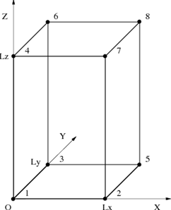
Let's create a block shape by combining six polygons using plot3d command. We first consider the case where one of the vertices coincides with the origin of the coordinate system and each side is parallel to the coordinate axis as shown in Figure 1 (we call this the "basic configuration"). In this case, if the length of each side (Lx, Ly, Lz) is given, the coordinates of the eight vertices are obvious. The six faces are defined by the following six sequences of vertices.
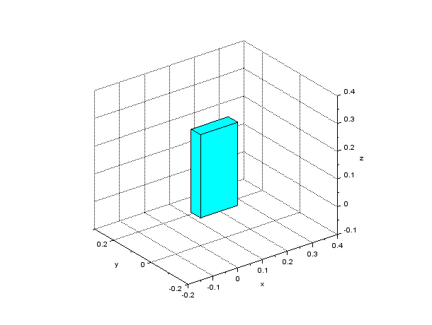
A Scilab script to draw a block shape in the basic configuration is shown in Code 1. The result of the drawing by this script is shown in Figure 2. Function genpat() used in the script is a function defined as in Code 2 that generates patches data, which is the input to plot3d, from vertices and faces matrices.
// make_block_special.sce

clear; xdel(winsid());

exec('genpat.sci', -1);

// Side lengths
Lx = 0.15;
Ly = 0.05;
Lz = 0.30;

// Vertices
vertices = [
    0,   0,  0;  // #1
    Lx,  0,  0;  // #2
    0,  Ly,  0;  // #3
    0,   0, Lz;  // #4
    Lx, Ly,  0;  // #5
    0,  Ly, Lz;  // #6
    Lx,  0, Lz;  // #7
    Lx, Ly, Lz]; // #8

// Faces
faces = [
    1, 2, 5, 3;  // #1
    1, 3, 6, 4;  // #2
    1, 4, 7, 2;  // #3
    4, 7, 8, 6;  // #4
    2, 5, 8, 7;  // #5
    3, 6, 8, 5]; // #6

// Patches
patches = genpat(vertices, faces);

// Draw patches
h_fig = figure;
h_fig.background = 8;
h_pat = plot3d(patches.x, patches.y, patches.z);
h_pat.color_mode = 4;
h_pat.foreground = 1;
h_pat.hiddencolor = 4;

// Axes settings
xlabel("x"); ylabel("y"); zlabel("z");
h_axes = gca();
h_axes.isoview = "on";
h_axes.box = "off";
h_axes.rotation_angles = [63.5, -127];
h_axes.data_bounds = [-0.2, -0.2, -0.1; 0.4, 0.3, 0.4];
xgrid;
function patches = genpat(vertices, faces)
// Generate patches data from vertices and faces
patches.x = vertices(:,1)(faces');
patches.y = vertices(:,2)(faces');
patches.z = vertices(:,3)(faces');
endfunction